
An Examination of MLX Quantization
Empirical scaling laws, surprising results, and an esoteric quantization recipe.

Note: The chronological order of this exploration has been rewritten for the sake of the reader.
Recently, I’ve been experimenting with a variety of quantization settings in MLX, and documenting intriguing empirical results. This particular adventure started w/ the release of Qwen3-4B-2507-Instruct, a SOTA 4B model. The standard 4bit quant in MLX ran at 120tok/sec+ on my device, so I wanted to see just how much performance I could pack into a quant that would run at similar speeds.
To start my exploration, a brief summary of MLX quantization:
MLX quantization has two primary parameters - call them Q_BITS (bits) and Q_GROUP_SIZE (group size). The quantization algorithm employed is fairly simple - split every tensor up into Q_GROUP_SIZE groups, and for each group, calculate the min and max. Then the interval is divided up into 2^Q_BITS bins, and each weight is mapped to a bin. This uniformly distributes the available precision across each group, and requires only storing two floats (typically in bf16) as per-group parameters (a scale - corresponding to the interval each bin covers and a bias - corresponding to the min or max, whichever has larger magnitude). The actual algorithm is slightly more in-depth than this (it has special handling at the edges of the interval), and interested readers can check it out here.
This quantization scheme gives us a fairly compact formula for the overall bits per weight of a quant, taking into account Q_BITS and Q_GROUP_SIZE:
BPW = Q_BITS + (32/Q_GROUP_SIZE)
The standard 4bit quant uses a group size of 64, giving us 4.5 BPW by default. The question then becomes: in a similar amount of BPW, how much performance can we maintain?
First, how to evaluate performance? Due to the constraints of quantizing and evaluating on an M3 Max, we’ll forego benchmarks and simply evaluate perplexity on a reference corpus. For the rest of this blog post (with certain exceptions), I’ll be referencing perplexity values computed on enwik8 via a simple methodology: evaluate perplexity on 256 random sequences of 512 sequential tokens from the reference corpus, and average.
We can start by varying Q_BITS from 3 to 8 (as 2 outright breaks the model, >10000 ppl), and fitting a curve to the resulting perplexity, with BPW as the input:
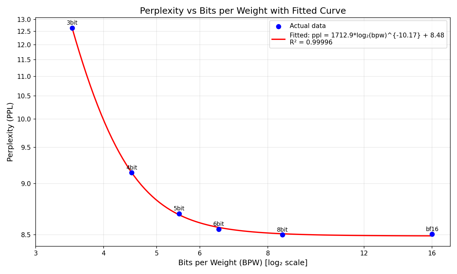
The quantization behavior is extremely predictable, with a simple three-parameter model a*log2(bpw)^b+c achieving an R^2 of 0.99996 when fit to the 6 points we have. Intriguingly, this power-log law surpasses the more conventional a*2^(-b*bpw) + c - getting a BIC (lower is better) of -50.0661 compared to the exponential’s -36.9275.
Qualitatively, the curve matches intuition - the 8bit quant is essentially lossless (matching the ~8.5 ppl of the bf16), there’s a tiny bit of loss at 6bit, a little more at 5bit, over 0.5 ppl of degradation at 4bit, and the 3bit degrades to 12.6 ppl. (Note that all stderrs are ~0.1 - meaning statistical significance is called into question for extremely close comparisons. For the rest of this blog post, we’ll focus soley on the raw means as the goal is to get as low a perplexity as possible. But the lack of statistical testing means this blog post shouldn’t be taken as a properly proved recipe.)
Given this baseline, how can we improve things? MLX provides a whole variety of “learned quant” techniques - the most popular of which is DWQ (Distilled Weight Quantization) - an ingenious method which takes advantage of the fact that the aforementioned scales and biases are continuous floating point numbers - which means they can be optimized via gradient descent. DWQ optimizes these scales and biases to minimize both the KL divergence and MAE of hidden states with a reference model - typically the original bf16 model. DWQ is normally applied as a post-processing pass on an existing quant, with the scales & biases already initialized by the min-max scheme described above.
The issue for experimentation is that DWQ introduces a slew of new hyperparameters - learning rate, number of tokens, but most importantly, the calibration dataset. The default calibration dataset MLX uses is the extremely rich tulu-3-sft-mixture, which contains a diverse variety of conversations. However, this is off-policy data - the model that generated these conversations is not Qwen3-4B-2507-Instruct. So I rented an H100 from Hugging Face for 20 minutes (very cheap, <$2) and generated a set of 1024 completions to user prompts from the tulu-3-sft-mixture using Qwen3-4B-2507-Instruct. This let me set up a controlled experiment - train the model on the off-policy and on-policy completions, and see which one has better resulting perplexity.
Surprisingly, the off-policy DWQ got a ppl of 8.78 compared to the 8.84 of the on-policy DWQ. Thus, for all other quantization experiments, off-policy DWQ will be used. Applying DWQ to the 3, 4, 5, and 6 bit models (with the lossless 8bit and bf16 included) yields the following curve:
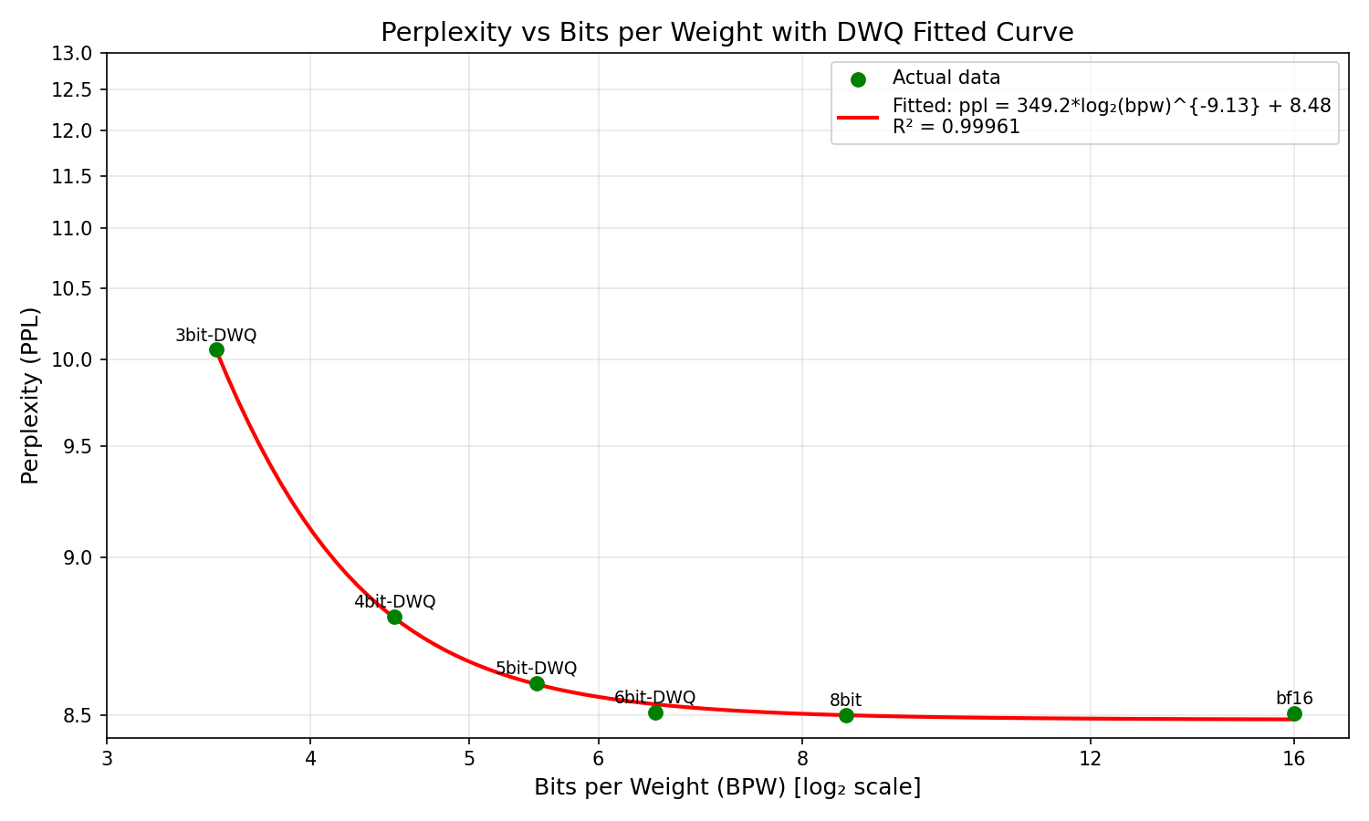
The inverse log power law is slightly less explanatory here (BIC of -48.6366), but still slightly beats the exponential alternative (-47.6467). Most notable is the drop in the coefficient of the log2 - from 1712.9 w/out DWQ to 349.2 with - indicating the perplexity grows far less steeply. See here side by side:
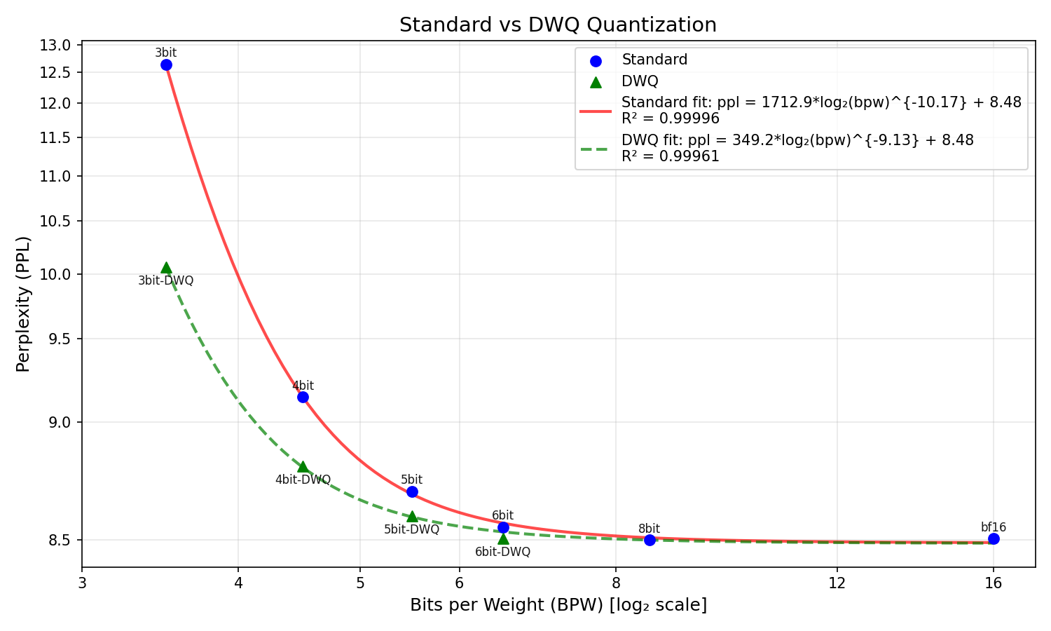
I suspect the reason the DWQ curve is less explanatory is because I had to eyeball learning rates for the DWQ process based on the perplexity of the quant - I varied the LR from 2e-7 to 1e-6 and had to do so based off intuition as I lacked the compute for a full sweep (I found 2e-7 worked well for 6 and 5 bit, 1e-6 for 4bit, and 2e-6 for 3bit). A proper sweep may reveal a more predictable pattern.
However, we can do a cool thing with the pattern we do have - we can find the ‘effective BPW’ that DWQ adds to the model. Math justification below - skip if you want the effective BPW added:
For a given bpw x, the DWQ curve predicts a ppl of 349.2*log2(x)^(-9.13) + 8.48. We can then find the ‘non-DWQ’ bpw associated w/ that ppl using the standard log2 fit, which is 1712.9*log2(x)^(-10.17) + 8.48. Invert that and pass in the DWQ curve to get a function that maps any DWQ bpw to the ‘normal’ bpw - which works out to 2^(1.1693*log2(x)^0.8977). Subtract x to get the difference from the DWQ quant. This obviously is non-constant, so we’ll get the average value over the quantization domain that interests us - 3.5bpw to 6.5bpw. This can be done via integral + mean value theorem.
This works out to an effective 0.613 bits that the off-policy DWQ adds to the quantization quality of our model - roughly 0.47 bits at 3.5 bpw and 0.72 bits at 6.5bpw. In other words, a DWQ at bpw X is roughly equivalent to a standard quant at bpw X + 0.613.
After experimenting with DWQs, I moved on to another learned quantization method MLX has - the simpler dynamic quant. This technique uses a calibration dataset as well, but instead of optimizing the scales and biases directly, it instead computes per-tensor sensitivities by analyzing the importance of each tensor is reducing KL divergence as well as the absolute difference between the tensor quantized at low and high bit values. The sensitivities are then used to quantize the model to a target BPW by assigning some tensors to a pre-set ‘low’ quantization scheme (say, 4 bits) and others to a pre-set “high” quantization scheme (say, 6 bits). The resulting model can then be used out-of-the-box, or as an initialization for a DWQ.
While I won’t go as in-depth with my experiments with dynamic quants, I tested a variety of methods at 5bpw and found that the one that reduced perplexity the most was the strange scheme of computing sensitivities using a 3bit quant as the ‘low’ setting and a 5bit quant as the ‘high’, but then actually quantizing the model with 4bits as the ‘low’ and 6bits as the ‘high’. This resulted in a model that achieved a ppl of 8.75. This outperforms the 8.85 ppl the naive 5bpw quanting strategy gets (4 bits with a group size of 32).
This dynamic quant can then be DWQ’d (I’ll call this the DDWQ) - after which it achieves a perplexity of 8.64, which is again significantly lower than the DWQ’d naive 5bpw quant, which gets 8.70. For quality reference, 8.64 is lower than the normal 5bit (5.5bpw) quant’s 8.67 - which checks out, as we should expect DWQ’s to add ~0.6bpw to overall quality, and a ppl of 8.64 corresponds to a bpw of 5.62 by the curve fitted above.
This data suggests that while the dynamic quant is capable of producing a model that complies with our empirical DWQ curve, the naive 4bit-32gs does not (8.7 only corresponds to 5.33bpw, not the 5.6bpw we’d expect). This led me to wonder whether the Xbit-32gs models even fit along our original curve - given that the mechanism by which more precision is added (halving the group size instead of doubling the bin count) is entirely different. The plot showing how the 32gs models lie along our curve is below:
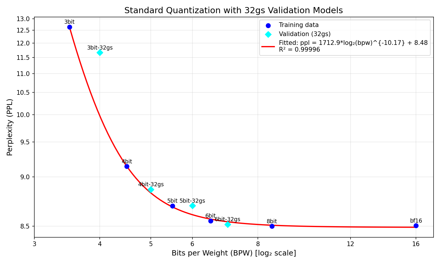
The results are interesting - the 4bit-32gs and 6bit-32gs lie somewhat along the curve, the 5bit-32gs is slightly off, and the 3bit-32gs is wildly off, scoring over 1.5 ppl higher than predicted. A tentative conclusion could be that 32gs is more effective at even-bit quantizations - but this would require far more research to verify.
Finally, one graph with all of this analysis together:
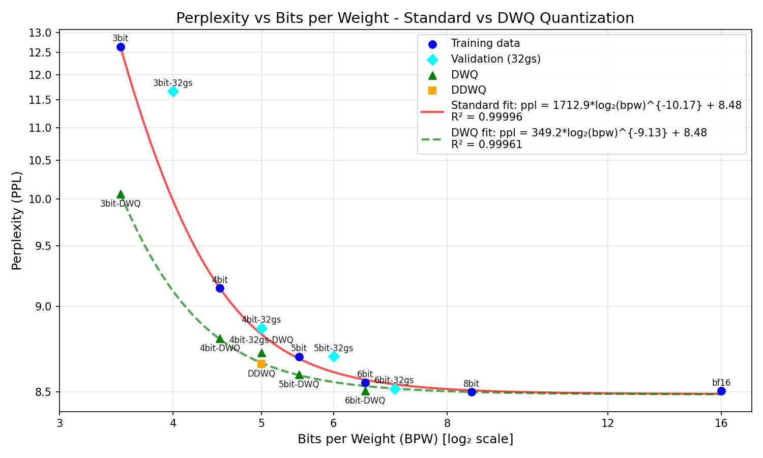
The plot above combines all the insights - how DWQ shifts the bpw-ppl curve downward, the half-decent fit of the standard quant’s curve to the 32gs data, and the power of the DDWQ model.
Now, back to my original question - how much performance can I pack into a quant that would run at similar speeds to the 4bit quant? The true answer is the 4bit-DWQ - dynamic quantization requires a BPW >4.5 to be effective. But if we loosen the constraints to include 5bpw models, then the DDWQ fits perfectly along the DWQ pareto frontier at 5bpw. Speed-wise, the DDWQ runs at 110 tok/sec on an M3 Max, right between the 5bit (100 tok/sec) and 4bit (120 tok/sec). Thus is the end result of my tinkering: a model that runs almost as fast as the 4bit quant and performs better than the 4bit-32gs-DWQ (the naive approach at 5bpw). The model is available on Hugging Face here.
However, I think this end result is probably the least interesting part of this exploration overall - I was far more intrigued by the inverse log power law that fit the standard quantizations so well, and how that somewhat transferred to the DWQ data. Further research (that I might do myself) could explore to what extent this generalizes to other models - do all Qwen models follow this sort of bpw-PPL relation (this is the lowest-hanging fruit)? What about models of other families? Is it a property of MLX quantization or can it be replicated w/ llama.cpp? Does DWQing models always enhance the pareto frontier by a consistent amount of effective bits per weight?
The evidence I have suggests the picture is far more complicated across different model scales - my previous work with DWQing larger models (Qwen3-30B-A3B) showed a 4bit DWQ outperforming a 6bit-32gs, which is wildly inconsistent with the modelling established here. A further issue with the methodology here is the eyeballing of DWQ learning rates - LR sweeps would be necessary to get a true idea of the minimum DWQ loss at each bit count.
Thus concludes my exploration of various quantization techniques in MLX - for anyone skimming the article, a quick tl;dr of tips and counterintuitive results:
DWQ on the default dataset is better than DWQ on on-policy data
DWQ tends to be equivalent to a 0.5-0.6 increase in the bpw
Dynamic quantization works better for 5bpw quants than 4bit-32gs
Dynamic quantization can be further enhanced with DWQ
The relationship between bpw and perplexity for Qwen3-4B follows an inverse log power law
Thank you for reading, and may your quantizations be fruitful!
An error in code underestimated standard errors by an order of magnitude. This has since been rectified and a disclaimer attached.